The smartest ML approach to forecast loan disbursals with accuracy

Building ML forecasting model: What happened since day 1

We started with problem scoping, unravelling two years of data and expanding the problem statement in detail—which turned out to be more nuanced than expected.

Their ask was simple: “Can we estimate this month’s total two-wheeler loan disbursals by the 15th, so our business heads can act fast and hit targets?”

Alongside this, they also wanted to understand:

• What factors drive disbursal volumes?

• Can we break this down by region, product, or customer profile?

We started with understanding their requirements:

• Types of loans, customers, focused regions, festivity and seasonality

• Forecasting frequency

• What exactly needs to be forecasted and more.

A simple case of machine learning forecasting that became a multi-disciplinary effort, drawing out our skills from all areas: deep domain understanding, extensive data engineering, advanced modeling, and post deployment tuning.

Data complexities and other challenges in modern forecasting

Complex data landscape

Data is the most crucial part for any machine learning and forecasting project. The client we worked with had shared 2 years of historical data to begin with, collected from multiple touch points.

• Leads from showroom CRM systems

• Funnel stages: Logins → Leads → Sanctions → Disbursals

• Meta-data: Region, Customer type, App score, Product info

• External & campaign factors: Dealer count, Holidays, Promotions, Incentives, Interest Rate of Return (IRR)

We encountered some inconsistencies, quality issues, and schema differences.

• Each source had its own schema, format, and refresh cadence.

• Unstructured texts, unclear labels, and missing values.

We spent a good amount of time cleaning up data, standardizing IDs across systems, and defining rules for imputing values vs. discarding rows.

Too many disbursal patterns

Secondly, forecasting disbursal data didn’t exhibit a straightforward pattern.

We weren’t forecasting one time series. We had hundreds of combinations (e.g., region × product × customer score group) each with its own disbursal pattern. Other factors like forecast logins and sanctions needed to be predicted as well for accurate forecast disbursals.

Have to reduce dimensionality

Not focusing and fixing the fragmented forecasting can lead to errors. Our focus here is to get better accuracy and avoid errors. That’s why we decided to reduce dimensionality.

The technique we took to reduce noise and dimensionality was clustering. We chose four key dimensions to cluster across:

• Region

• Product group

• Customer profile

• App score

Based on the data, we identified 6 distinct clusters, each showing a meaningful pattern in disbursals.

For example: We grouped 14 regional codes into 2 broad clusters using correlation-based clustering. This grouping preserved pattern similarity, reduced dimensionality, and helped us build more stable and scalable forecasting models.

And there were many similar challenges like this that we solved while strategizing our forecasting approach, building, and validating it.

Building forecasting ML model with accuracy

Identifying key drivers

For accurate and more explainable forecasting reports, identifying key drivers (both internal and external) is instrumental. Like a new policy change or a dealer strike, in the case of an insurance business.

Our team identified over 20 potential external drivers influencing disbursals: some of which are dealer strength, IRR, promotions, holidays, and sales incentives, apart from those that the client shared.

We used a Random Forest Classifier to shortlist which features mattered most for high vs low disbursal periods. The reason for using the random forest classifier was the presence of non-linear combinations, its agility against overfitting, and the need to comprehend complex patterns.

Forecasting approach

Now we have the data, clusters, external drivers, and everything needed for forecasting, except for one thing – the second half of the month’s input values. Here’s what we did.

Use separate models to predict and fill the missing values - like no. of leads or logins. Predict the disbursal rate for each cluster using algorithms like:

• Random Forest Regressor

• XGBoost Regressor

Evaluating forecasting performance and accuracy through validation

The next is the validation stage, where we identified how well the model may work for a new set of data. Validation is a must in order to prevent overfitting issues, select the best fitting model, and tune hyper-parameters if necessary.

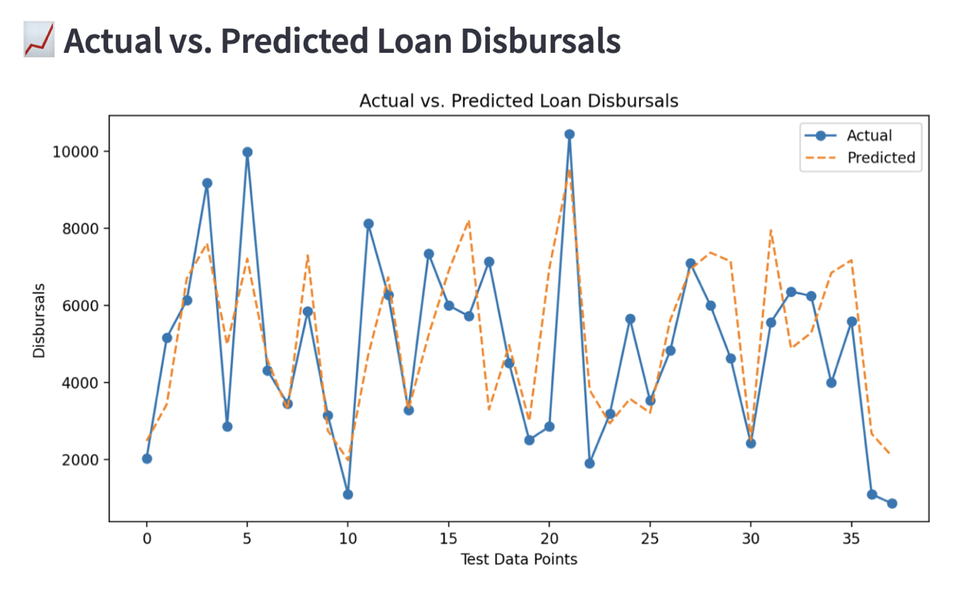
We used the last few months as a validation set, evaluating model performance using metrics: MAPE (Mean Absolute Percentage Error) and SMAPE (Symmetric MAPE). Both of these metrics explain how far off the predicted values are from the actual values.

A little side note about using MAPE and SMAPE as model validation metrics:

Most clusters showed reasonable predictive accuracy, especially for high-volume regions, which you can observe from the graphs below:

MAPE provided a straightforward understanding of average forecast error in percentage terms. But we couldn’t depend on it alone for low-volume markets, where even small absolute deviations inflated the error disproportionately. Hence, we had to use MAPE with SMAPE metrics together for more balanced insights. If your priority is to maintain fairness in evaluation, the combined approach will be better. Especially where under-forecasting could lead to under-serving demand, and over-forecasting could affect organizational operations and inventory planning.

Deploying the model in the live environment & monitoring performance

The next step is to deploy the model and monitor its functioning. This setup would empower decision-makers mid-month, enabling data-driven decisions to optimize promotions, dealer engagement, and incentive planning.

We used tools like Python (scikit-learn, XGBoost, pandas), Jupyter Notebooks, Streamlit, and MLflow in this stage. A successful deployment takes the following steps to happen:

• Deploy the model with monthly reports for business heads

• 2-3 months tracking to assess live accuracy

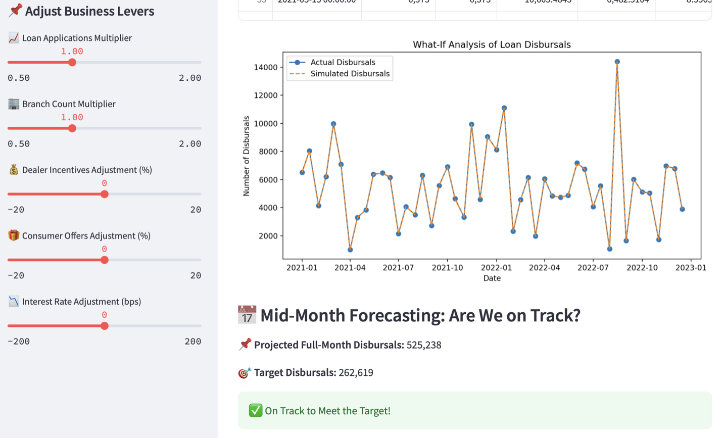
Attaching the screenshot that showcases the forecasting tracking UI operated by the business leads:

The UI image shows how there are different business levers enabled, which adjusted, will also alter the what-if analysis of loan disbursals.

Sharing a quick checklist for proper model deployment

• Ensure model readiness for live environment and set up validation metrics to suit the business forecasting accuracy requirements. (In this case it was (e.g., MAPE < 10%, AUC > 0.85).

• Package and version models in a standardized format for smooth deployment.

• Containerized or cloud-native infrastructure (e.g., SageMaker, Lambda) to scale efficiently.

• Dashboards and alerts for real-time monitoring.

Final thoughts

This PoC showed that even with limited data and noisy operational variables, a well-thought-out forecasting framework can deliver actionable insights. By clustering wisely, selecting the right variables, and forecasting in layers, we helped our client move one step closer to predictive decision-making in a competitive vehicle finance market.

Do you have similar requirements, or do you need data science consulting and assistance? Book a call with us to have an exclusive discovery session with our data science team.