A deep dive into time series forecasting techniques

What is time series data?

Time series data is a set of data points collected in chronological order at regular intervals. It is standard and widely used in many different fields such as economics, business, and weather forecasting. To be able to understand a time series, we must first understand the main components it consists of.

The components of a time series are the seasonal trend, cyclic trend, upward and downward trends, serial correlation, and non-linear trends. The seasonal trend is a repetitive pattern that occurs over shorter terms such as days, weeks, or months. The cyclic trend is a pattern that occurs periodically over a longer term such as years or decades. An upward or downward trend shows a gradual upward or downward change. Serial correlation shows a relationship between the adjacent data points. Lastly, non-linear trends are complex patterns that are difficult to predict.

By understanding the components of time series data, data analysts and scientists can more accurately forecast time series data. This allows businesses to make more informed decisions based on their data, which leads to better outcomes.

What is time series forecasting? 

Time series forecasting is about analyzing chronological data points to make interesting revelations about the future data points. Time series data is usually versatile and has applications across different fields, such as finance, meteorology, economics, and more.

Components of time-series data

Trend: long-term movement of data across time series

Seasonality: Patterns that repeat over time at proper frequency

Cyclical patterns: Fluctuations in data happen at irregular intervals due to factors like economic conditions. 

Irregular events: random noise that doesn’t fit into other components.

How does time series forecasting work?

Here is how you can analyze time series data to forecast future data points.

Decomposition: Break your time-series data into components (Trend, seasonality, cyclical patterns, and irregular events).

Stationarity testing: Perform stationarity testing to check if the statistical properties of time series data (mean and variance) are the same across the time. 

Model selection: Every data set is different. Upon understanding your data and its nature, select a suitable forecasting model.

Here is how you can decompose your time series data and find stationarity.

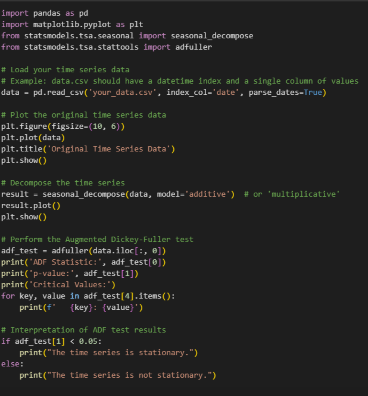
Methods to check Stationarity

There are many methods to check whether a time series (direct observations, residuals, otherwise) is stationary or non-stationary. Examine Plots

You can review a time series plot of your data and visually check if there are any obvious trends or seasonality. Summary Statistics

Reviewing summary statistics is a quick and dirty way to determine if your time series is non-stationary. You can compare the mean and variance of each group by dividing your time series into two (or more) partitions. The time series is probably non-stationary if they differ and the difference is statistically significant.Running the above instances reveals mean and SD values for each group that are once more comparable but not identical.We might conclude that the time series is stationary based solely on these data, but This is a quick and dirty method that may be easily fooled. Statistical Tests

We shall employ a statistical test to specifically comment on whether a univariate time series is stationary or not.

1) Augmented Dickey-Fuller (ADF) Test

2) Kwiatkowski-Phillips-Schmidt-Shin (KPSS) Test

3) Phillips-Perron (PP) Test

Algorithms in time series forecasting

Following are some of the algorithms used in time series forecasting. 

ARIMA(AutoRegressive Integrated Moving Average)

ARIMA is one of the most used forecasting models which works on a main goal of making the data stationary. It aims to achieve consistency, controlling the effect of seasonality. It has three components, AR stands for Auto regression, I stands for Integrated, and MA stands for Moving Average.

Auto Regression (AR): A statistical and mathematical technique that uses the relationship between an observation and number of lagged observations.

Integrated: The difference between the above observations is used to make the time series data smooth and stationary.

Moving average: Utilizes the relationship between an observation and the residual error of the moving average model applied to lagged observations.

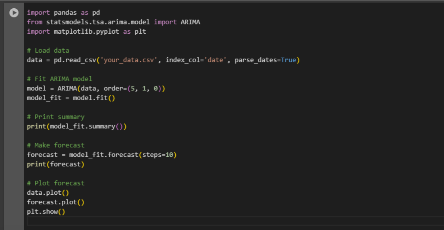
Use the following Python script to run ARIMA model after stationarity testing.

Exponential smoothing (ETS)

Exponential smoothing aka ETS (Error, Trend, Seasonal) is another popular forecasting technique. It relies on weighted averages of past observations, assigning exponentially decreasing weights as the observations get distant.

Depending on the time series data used, ETS can be classified into three types.

Simple exponential smoothing: Simple exponential smoothing is used for data that exhibits no trend or seasonality.

Linear trend model: You use Holt’s linear trend model for the time series data with a linearly distributed trend.

Holt’s winter seasonal model: When the time series data exhibits both trend and seasonality, winter seasonal model is used.

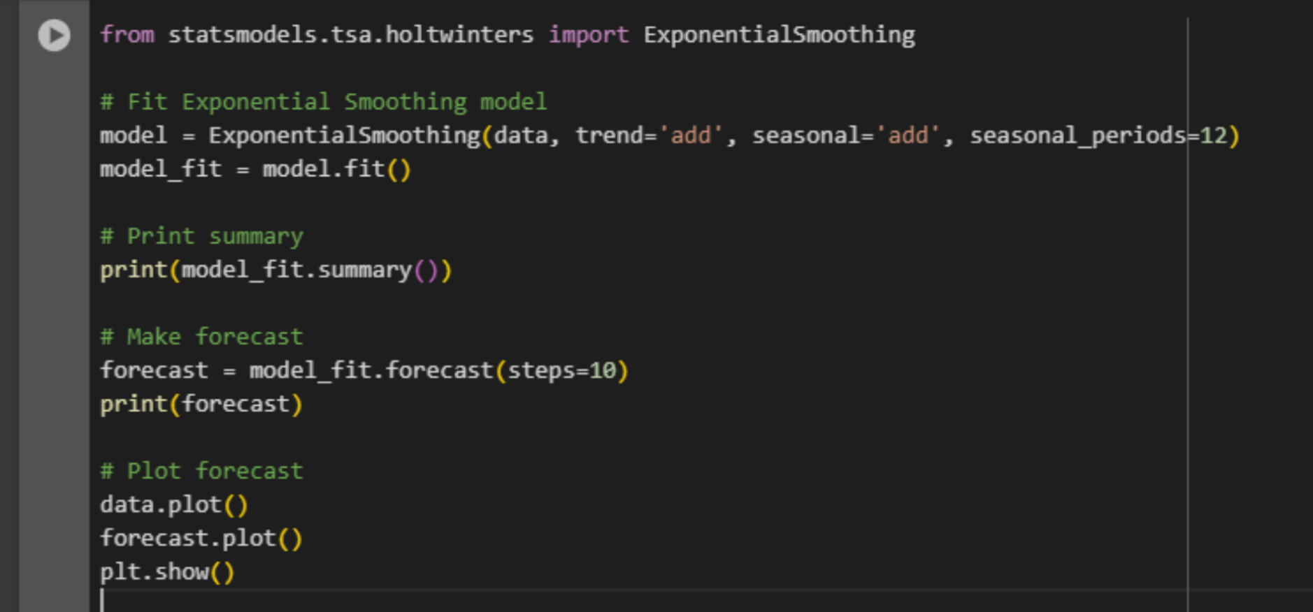
Use the following Python script to run exponential smoothing on the decomposed data.

Prophet

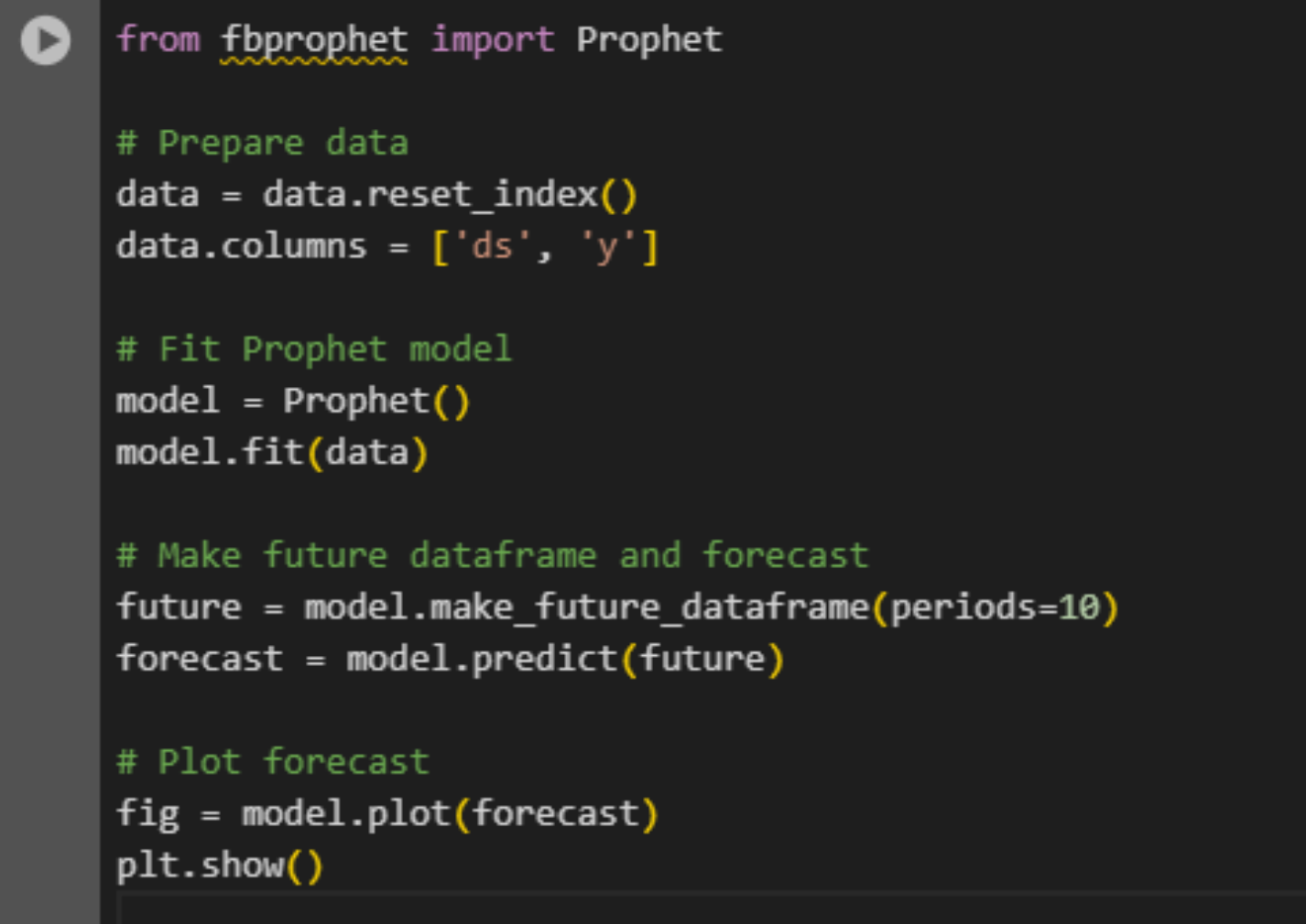
Prophet is a powerful forecasting tool by Facebook used for time series forecasting. You can use the Prophet model when there is a strong seasonality and missing data as it’s designed specifically for time series data with seasonality and outliers.

After decomposition and stationarity testing, run the following script to use the Prophet model for forecasting.

LSTM (Long Short-Term Memory)

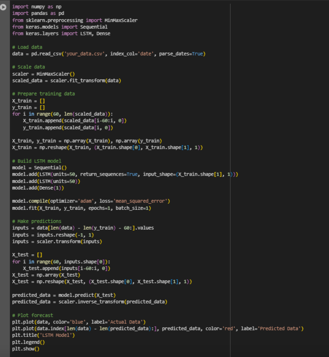
LSTM is a recurrent neural network which is perfect for complex time series data with long-term dependencies. Many stock market prediction models already use this neural network type forecasting technique as they learn long-term trends from the data.

You can run the LSTM forecasting model in Python using the following way.

SARIMA

SARIMA is an extended version of ARIMA which adds seasonality to capture seasonal effects in data. The model is denoted by (p, d, q)(P, D, Q, s), each denoting the following terms:

p : the number of observations in the model (Auto regression)

d : the number of times the raw observations are differenced (integrated part)

q : the size of moving average window

P : the number of seasonal autoregressive terms

D : the number of seasonal differences

Q : the number of seasonal moving averages

s : the number of steps for a single seasonal period

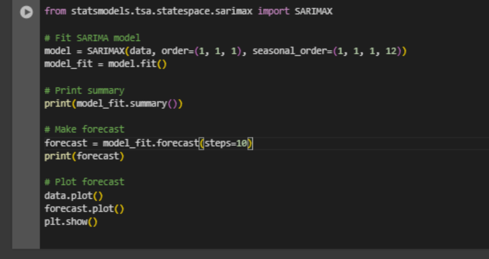
The major difference between ARIMA and SARIMA is that SARIMA includes additional differencing to remove seasonality by subtracting the value from the previous cycle’s corresponding season. It later involves fitting both seasonal and non-seasonal parts of the data. SARIMA model finally generates the forecast by combining fitted seasonal and non-seasonal components.

Here is how you can run the SARIMA model after decomposing the data.

Techniques to improve forecasting accuracy

Achieving accuracy in forecasting is crucial for forecasting models. Techniques like data prepossessing, feature engineering and fine tuning can help you improve forecasting accuracy.

Data preprocessing: Before forecasting, it is important to pre-process the data and clean by removing or imputing missing values. Other techniques like smoothing the noise and variables' transformation also improve forecasting accuracy.

Feature engineering: Using lags or moving averages, you can create new features from the existing time series data and it can improve accuracy and reliability of the forecast model.

Model fine tuning: This involves tuning hyperparameters of the model to capture the underlying patterns in the data.

Evaluating a forecasting model

Some of the commonly used statistical tests for time series forecasting are:

Mean Absolute Error (MAE): This is a measure of the average absolute difference between the actual values and the forecasted values. A lower value of MAE indicates better accuracy of the forecast.

Mean Squared Error (MSE): This is a measure of the average squared difference between the actual values and the forecasted values. A lower value of MSE indicates better accuracy of the forecast.

Root Mean Squared Error (RMSE): This is the square root of the MSE. It provides a measure of the average magnitude of the forecast error. A lower value of RMSE indicates better accuracy of the forecast.

Mean Absolute Percentage Error (MAPE): This is a measure of the average percentage difference between the actual values and the forecasted values. A lower value of MAPE indicates better accuracy of the forecast.

Final thoughts

Understanding time series data and its components and using its effective forecasting techniques will help businesses make better decisions and run smooth operations despite uncertain situations. Many industries like finance, healthcare, manufacturing, and logistics, use their time series data to predict demand, sales, and many unpredictable future events. They not only stay prepared for the future but also improve their bottom line without performing too much data analysis.

Want to build a business or process-specific forecasting model like them? Or improve forecasting accuracy of your existing model? Share your concerns with our data science experts and find feasible solutions exclusive to your business. 

📖 Recommended read: Read our customers’ story on how they achieved sales targets with loan sales forecasting.